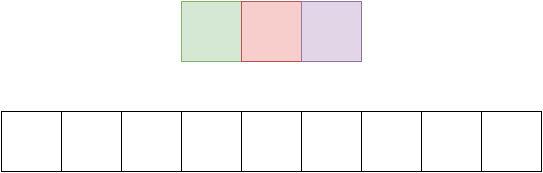
One thing that confuses newcomers to the C language, whο usually are newcomers to programming altogether, is the distinction between pointers and arrays. When you start learning C, you first learn about arrays. Every book or course teaches you statically allocated one dimensional arrays first. A statically allocated array is declared like this:
int array[10]; //Declares an array of 10 integers
One thing that confuses newcomers to the C language, whο usually are newcomers to programming altogether, is the distinction between pointers and arrays. When you start learning C, you first learn about arrays. Every book or course teaches you statically allocated one dimensional arrays first. A statically allocated array is declared like this:
int* dynamicArray= malloc(8*sizeof(int));
Let’s dissect the above statement. We have a pointer to an integer (array). If you’ve studied pointers, you know very well that a pointer to an integer is actually an integer itself that contains the address of an integer in memory. What happens next is that we use the malloc function that allocates memory for 10 integers on another memory segment, the heap. A ‘stack vs heaps argument’ could have an article on its own, but for now let’s just focus on the key difference between the two, which is the fact that everything that’s put on the stack lives as long as the function that created it lives. When that functions’ job is done, it gets kicked out of the stack and so are any variables, arrays or structures that were defined within it. On the contrary, everything allocated on the heap lives as long as the whole program lives in memory, unless we explicitly free that part of the memory. That’s another essential part of dynamic arrays that we are usually taught˙ when we’re done with them we should ‘free’ them:
free(dynamicArray); //Any memory that was used for this array now belongs to the operating system to utilize
The first question that popped into my mind when I started learning that stuff was: “How the hell can I tell the difference between a pointer to a single integer and a dynamically allocated array of who-knows-how-many integers?”
The missing piece of the puzzle was a small bit of information about arrays:
The name of the array (a.k.a the variable) is a pointer to the first element of the array.
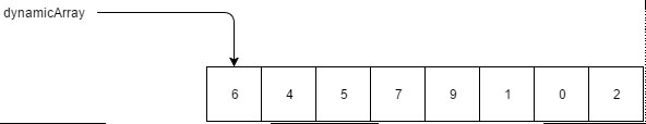
Sounds confusing? Let me explain. The variable that you use to handle the array, like ‘dynamicArray’ in the above example, is actually a pointer to the first element of the array. Let’s say that our dynamicArray contains the following integers: 6,4,5,7,9,1,0,2
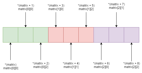
So we can get the first element just by dereferencing the pointer:
printf("First element = %d\n", (*dynamicArray));
Now, what about the second element? We can get that by moving the pointer one position to the right:
printf("Second element = %d\n", *(dynamicArray + 1));
The third element by moving two positions to the right:
printf("Third element = %d\n", *(dynamicArray + 2));
etc…
This sounds similar to the zero-based indexing of a statically declared array. If we wanted to get the first element of the array, we statically defined in the beginning of this article we would use this syntax:
int firstElement = array[0];
When you first learn about the zero-based index everyone tells you “that’s the way it is” and you’re left wondering why this:
int firstElement = array[0];
Is better than this:
int firstElement = array[1];
Now you know the reason why. It’s because the variable name points to the first element. And guess what, this applies to statically defined arrays too!
You see, the ‘dereference method’ of accessing array elements is not exclusive to arrays created using malloc. You can use it in plain old statically defined arrays too! Because the ‘array’ variable we used above is also a pointer. To better explain this, I’ve put together a small console application that shows that you can use both the indexing operator ( [] ) and the pointer dereference operator ( * ) with any array, whether statically or dynamically defined:
We start by defining two identical one dimensional arrays, the first one on the stack and the second one on the heap. We then go on and print the first and fifth element of each array using both methods, therefore proving that both methods can be used regardless of the way the array has been defined.
How to pass arrays as arguments
Now that we’ve dug deeper in the world of one dimensional arrays, let’s see how we can pass them around functions. To do that, let’s write a ‘printArr’ function that will print the contents of a one-dimensional array.
For a function to print an array, it needs to know two things: the array (duh) and its size. So we need a function that will take two arguments and since it won’t return anything, it can be void. So we have the function’s signature!
void printArr(int array[], int size);
The ‘[]’ syntax tells the compiler that this function expects its first argument to be an array.
Here’s the implementation. Nothing fancy, just a loop over the array contents and a call to printf
Now let’s use it to print the two arrays we defined earlier:
printf("Array contents:\n");
printf(array, 8);

printf("dynamicArray contents:\n");
printArr(dynamicArray, 8);
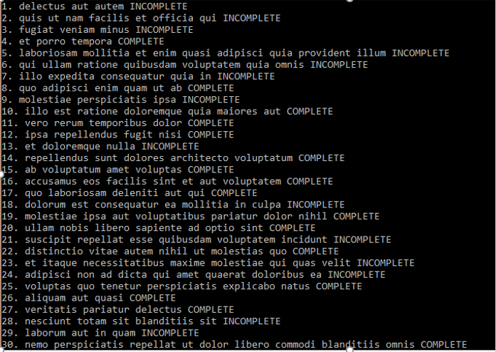
The results are:
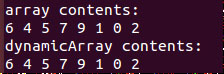
Which is correct, of course.
There is also another way to pass an array to a function. Instead of using the [] syntax, we could just pass a pointer since every array is actually a pointer to the first element!There is also another way to pass an array to a function. Instead of using the [] syntax, we could just pass a pointer since every array is actually a pointer to the first element!
There is also another way to pass an array to a function. Instead of using the [] syntax, we could just pass a pointer since every array is actually a pointer to the first element!
printf("Array contents (alternative method):\n");
altPrintArr(array, 8);

printf("dynamicArray contents (alternative method):\n");
altPrintArr(dynamicArray, 8);
What should I use
Okay, so, we learned that there are two ways to access an arrays’ content and there also are two ways to pass an array to a function. But which one should I use? Well, when it comes to accessing array elements, I personally believe that using the indexer operator makes your code cleaner, nicer and more comprehensible. As far as argument passing is concerned, someone might say that the pointer approach can get confusing when someone else reads your code because there is no immediate way of telling if the function accepts a pointer to a single element or an array.
It all comes down to personal preference though. I personally prefer using the indexing operator for accessing elements and I like using the pointer syntax for array arguments.
Conclusion
That was it! I hope you found this article helpful in your quest to master not only one-dimensional arrays, but C in general. The rest of the code can be found on GitHub. More stuff on C coming up soon. Thanks for reading. Keep coding!!